Visualizing CNN Activations
Friday, May 22, 2020
Posted by Tushar Nitave, Dept. of Computer Science, Illinois Tech, Chicago
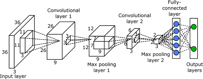
image source: https://www.codespeedy.com/wp-content/uploads/2019/05/convolutional-layers-of-an-image-Deep-learning-Machine-learning.jpg
In this post I will talk about visualizing CNN activations in python3 using a pre-trained neural network model. These activations are really helpful to see what each layer learns from a given image during training of the neural model. The output of the layers is called it's activation and these activations are nothing but feature maps that are output by various convolution and pooling layers.
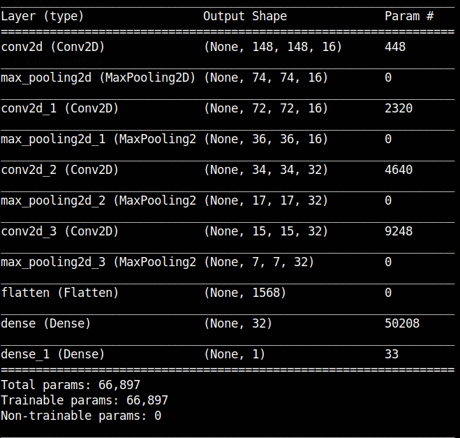
I will use a small model that I trained from scratch on cat-versus-dog dataset. Following image shows you the model summary of the trained model. You can see the names of different layers (conv2d_1, conv2d_2 etc.) and how the dimension of the image (Output Shape) decreases as it is passed through different convolutional and maxpooling layers.
Let's get started:
- Load the pre-trained model
- Preprocessing the input image
- Getting layers from the model
- Visualize the channels
- Results
model = load_model("model.h5")
model.summary()
input_img = "cat.jpg"
img = image.load_img(input_img, target_size=(150, 150))
img_tensor = image.img_to_array(img)
img_tensor = np.expand_dims(img_tensor, axis=0)
img_tensor /= 255.0
layer_outputs = [layer.output
activation_model = models.Model(inputs=model.input, outputs=layer_outputs)
activations = activation_model.predict(img_tensor)
first_layer = activations[0]
plt.imshow(first_layer[:,:,5], cmap="viridis")
first_layer = activations[1]
plt.imshow(first_layer[:,:,1], cmap="viridis")
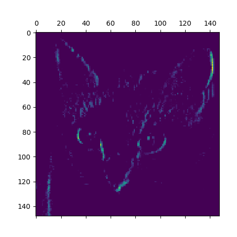
Fig 1: Fourth channel of first layer.
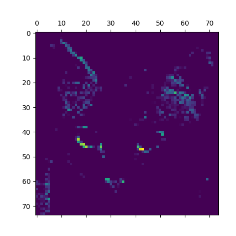
Fig 2: Second channel of second layer.
From fig 1 we can see that this filter is trying to detect edges in the image and in the fig 2 we can see that it is trying to detect eyes and ears. Each every channel encodes features independently.
Few things which we can conclude for CNNs are that, initial layers act as various edge detectors. They try to learn simple patterns. As we go deep in the network the filters try to encode higher-level concepts like detecting specific parts (eyes, ears etc.). Also, sparsity of the activations increases with increase in the depth.
This was a relatively small model with only 66,000 trainable parameters. If you train a bigger model or load bigger pre-trained models like VGG16, VGG19 etc. you can better visualization.
Note: I have shared the pretrained model —model.h5, requirements.txt and input image so that you can easly try it yourself. You can download it from here